In his book ‘Principles of Political Economy and Taxation’, David Ricardo, a British Economist said:
“A Country possessing very considerable advantage in machinery and skill and which may therefore be enabled to manufacture commodities with much less labour than her neighbours, may in return for such commodities import a portion of its corn required for its consumption, even if its land were more fertile, and corn could be grown with less labour than in the country from which it is imported.”
His subtle idea is the main basis for most economists’ belief in free trade today. The idea is based on the concepts of opportunity cost and comparative advantage.
Comparative Advantage and Opportunity Cost
Opportunity Cost is the cost of not being able to produce something else with the resources (i.e. human capital, time) used.
Comparative Advantage is the advantage of an entity in producing a good or service over the rest measured based on the opportunity cost.
Absolute Advantage is the advantage of an entity in producing a good or service over the rest measured based on the cost. (Generally more efficient in every production compared to any other parties).
Example: Suppose that the U.S. could produce 10 million roses with the same resources that could produce 100,000 computers. While Colombia could produce 10 million roses with the same resources that could produce 30,000 computers.
In this example, the U.S. has opportunity cost of 0,01 unit of computer when producing one unit of rose, and 100 unit of roses when producing one unit of computer. Meanwhile Colombia has opportunity cost of 0,003 unit of computer when producing one unit of rose, and 333,33 unit of roses when producing one unit of computer.
In other words, the U.S. has lower opportunity cost of producing computers and Colombia has lower opportunity cost of producing roses. In this regard, both countries have their own comparative advantage. When each parties have their own comparative advantage, they can trade to earn gain from each other.

By trading, the U.S. and Colombia together could for example produce and consume the same amount of roses, but 70,000 more computers.
Intuition: as long as each party has their own comparative advantage comparative advantage (lower opportunity cost), they can specialise their production and trade with each other to produce more goods and services at aggregate (world) level.
One-Factor Ricardian Model
The modern version of Ricardian model assumes that there are two countries producing two goods using one factor of production, usually labour. This model is a general equilibrium model, where flow of money in exchange for goods and services are in complete circle (supply equate to demand in all markets simultaneously).
The model incorporates the standard assumptions of perfect competition :
- Goods and services produced are homogeneous across countries and firms within an industry;
- There are no logistical costs in trading the goods and services;
- Labour productivity is homogeneous within the country but may differ across countries (implication: production technology, education systems, working environment may differ);
- Labour is free to move only across industries within a country without any costs;
- Labour market is at its full employment;
- Consumers (the labours) are assumed to maximise utility and consumption.
To be frank, to simplify the model analysis, we usually use Two Products produced in Two Countries using One Factor of Production (labour); each countries has Maximum Utilisation and Demand where both products are consumed in the same fixed proportion at given prices regardless of income.
The explanatory variable in this model is Labour Productivity : the quantity of goods and services produced by a worker during a unit of time (i.e. an hour). To indicate how productive workers in each country are, we can specify how much labour is required to produce a unit of final good.
Unit Labour Requirement indicates the number of hours of labor required to produce one unit of output. A high unit labour requirement means low labor productivity.
Production Possibilities Frontier (PPF)
Production Possibility Frontier (PPF) shows the maximum amount of goods that can be produced for a fixed amount of resources.
Example: Assume Home country produces only cheese and Foreign country produces only wine.

aLC : Labour required per unit of cheese
QC : Units of cheese produced
aLW : Labour required per unit of wine
QW : Units of wine produced
L : Available Labour
To find out the maximum production capabilities, we only need to divide the number of available labour by the number of labour required to produce one final product or service. For example, suppose that: L = 1,000; aLC = 1; aLW =2
The Production Possibility Frontier would be QC + 2QW = 1,000 while the maximum cheese and wine that can be produced would be 1,000 and 500 respectively.
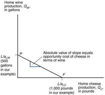
To calculate the opportunity cost of producing cheese, we just need to divide the unit labour requirement of cheese by wine’s. This will equal to the absolute value of slope of the PPF:

In the numerical example, if 1 hour of labour is moved from wine to cheese production, that additional hour could have been utilised to produce ½ unit of wine. Hence, the opportunity cost of producing 1 unit of cheese is ½ (slope of the PPF) of wine.
Relative Prices, Wages, and Supply
Relative price (or wage or supply) is a price of a good or service (or job) measured relative to the price (or wage or supply) of another good or services (or job). In short, it is an opportunity cost of choosing an alternative over the other.
Owing to the assumption that workers can move freely across industries, workers will choose to work in the industry that pays the highest wage.
Example: Assume PC is the price of cheese and PW is the price of wine. The hourly wage of cheese/ wine workers equals to the value of cheese or wine produced in an hour (PC/aLW).
In absence of trade, forces of demand and supply determine domestic production or consumption. Therefore, if the consumers want to consume both wine and cheese, prices must adjust so that wages are equal in the 2 sectors so workers will be indifferent to work in either sector:

or equivalently

In absence of trade, the relative price of a good will be equal to the opportunity cost of producing that good.
Trade In The Ricardian Model
The notations in Foreign country are usually denoted by the asterisk sign (i.e. L*). Since there is only one factor of production in the Ricardian model, a country’s advantage is based on the unit labour requirement (i.e. aLC or aLW) of producing a product or service. In real life, it is almost impossible for a country to have ALL comparative advantage.
Based on the example given above, before trade occurs, the relative price of cheese to wine reflects the opportunity cost of cheese in terms of wine in each country. When trade occurs however, there will only be one world market for both cheese and wine; which means there will only be one world relative price for each. This relative price is determined by forces of demand and supply.
When analysing comparative advantage after trade, we need to take into account what happens in ALL markets simultaneously (general equilibrium analysis). We can do so by analysing the relative demand and relative supply.

The thresholds on the Y axis are both relative unit labour requirement of home’s and foreign’s. In the X axis we put the WORLD relative quantity of cheese over wine.
When the relative price of cheese is below the opportunity cost of producing it, none of the country will produce cheese (from 0 to aLC/aLW).
When the relative price of cheese equals to home’s opportunity cost, home will specialise in producing cheese until its maximum relative production capacity (L/aLC)/(L*/a*LW).
As the price of cheese relative to the price of wine rises (demand curve relative to vertical part of supply curve), consumers in all countries will tend to purchase less cheese and more wine so that the relative quantity demanded of cheese falls. The same can be said for the production in both countries. As the price of cheese rises, the wage of producing cheese will also rise. That being said, when the wage reaches foreign country’s opportunity cost of producing cheese, they will be willing to produce cheese. Consequently, the relative supply of cheese will become infinite.
In general, the relative price of cheese after trade will fall between the relative prices (opportunity costs) of cheese in foreign and home before trade.
Ways To Observe Gains From Trade
1. Trade as a ‘better technology’
We can look at trade as ‘indirect production method’ that is more efficient (less costly) for both countries. That being said, a country can gain from trading by specialising their production on a product or service that they have comparative advantage over and exchange the output for the product of another country that produces the product or service that they need.
2. Trade as a way to extend Consumption Possibility Frontier (CPF)
Another way of observing gains from trade is by looking at how trade affects Consumption Possibility Frontier (CPF). Without trade, consumption possibility (CPF) will only equal to the production possibility (PPF). With trade, the possibility will be higher.

Relative Wages
Relative wages are the wages of a country relative to the wages of another country they are trading with. Note that relative wage (in Ricardian model) does not depend on the price of the product, rather on the productivity of the workers.
Numerical Example:

Suppose that PC = 12 and PW = 12
Since domestic workers specialise in cheese production after trade, their hourly wages will be PC/aLC = 12/1 = 12; since foreign workers specialise in wine production after trade, their hourly wages will be PW/aLW = 12/3 = 4.
The relative wage of domestic workers is therefore 12/4 = 3. Which means home country’s wage is 3 times higher than the foreign country’s wage.
From this illustration we can also observe that both countries have their own Cost Advantage in production:
Foreign country has their cost advantage from their lower wage in wine production despite lower productivity.
Home country has their cost advantage from their productivity in cheese production relative to foreign country’s, despite higher wages.
Model Implication : as long as each countries has their own comparative advantage, even though their productivities differ from each other, both countries can gain from trade.
Empirical Evidence : many studies have proven the positive correlation between wages and productivity. Below is a scatterplot that shows that a country’s wage rate is roughly proportional to the country’s productivity.

Comparative Advantage With Many Goods
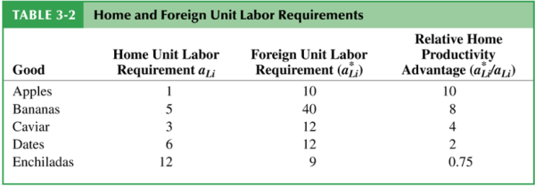
With many goods involved in trade, pattern of trade depends only on the ratio of Home to Foreign wages. Simply put, goods will only be produced where it is the cheapest to make them. In other words, the general rule is as long as the wage of producing that good is still higher than the relative Home Productivity Advantage (a*Li/aLi), produce at Home. Say relative wage per hour is 3, in this case, home will produce apples, bananas and caviar at Home and ‘produce’ the rest outside of the country.
In the two-goods model, we can determine the relative wages because we know who produces what based on their comparative advantages. In the multi-goods model however, we need to know the relative wages before we can determine who will produce what. To find these, we need to take a look at the derived demand that results from the demand for goods produced with each country’s labour (not the customers’ direct demand). In other words, it is determined by the relative supply and demand for labour services of each products. In the Ricardian Model, the supply of labour is assumed to be fixed (no immigration).

By putting the relative supply curve and the relative demand curve together, we can determine the equilibrium relative quantity of labour demanded in each country, equilibrium relative wage, and the production that occurs in each country.
In other words, these elements depend on the relative size of each country’s size (which determines the relative labour supply and the position of the RS curve) and the relative demand of the goods produced (determines the shape and position of the relative demand (RD) curve).
From this graph, we can see that whenever we increase the wage rate of the relative demand of Home workers relative to that of Foreign workers, the relative demand for goods produced in Home will decline and the demand for Home labour will decline with it. The flat lines correspond to relative wages that equal to the ratio of Home to Foreign productivity for each of the five goods. If the intersection of RD and RS happens to lie on one of the flat lines, both countries will produce the good to which the flat applies.
Transportation Costs and Non-Traded Goods
The Ricardian model predicts that country completely specialise in production (maximum one good produced by both). However, this rarely happens in reality for at least four main reasons:
- There is more than one factor of production. More factor of production will lead to reduction of tendency in specialisation;
- Protectionism. Government plays a major role in setting up barriers for trade (i.e. tariffs and quotas for certain goods or services);
- Transportation costs. In some cases, transportation costs are enough to lead countries into self-sufficiency in certain sectors of industry;
- Customers like variety. Take apple for example, although on the paper they all look the same, customers prefer to have options of what kind of apples they can buy.
Empirical Evidence of Ricardian Model
A study done in 1951 shows that U.S. exported goods to the U.K. that they have higher relative productivity over. The data confirms the model predictions, U.S. had an absolute advantage in all 26 industries, yet the ratio of exports was low in the least productive ones.

Another study in 1995 that compared the Chinese output and productivity with that of Germany for various industries also shows similar evidence. Chinese productivity (output per worker) was only 5 percent of Germany’s on average. However, Chinese productivity in apparel was about 20 percent higher of Germany’s.

From these empirical evidences, we can conclude that: Productivity differences play an important role in international trade; Comparative advantage (not absolute advantage) matters for trade.
Key Takeaways:
- Differences in the productivity of labor across countries generate comparative advantage;
- Comparative advantage is measured by the opportunity cost of producing that good. The country with the lowest opportunity cost, has the comparative advantage;
- When each country export goods that they have comparative advantage over, everyone can gain from trade;
- Empirical evidence supports trade based on comparative advantage, although transportation costs and other factors prevent complete specialisation in production.
References: Krugman, P.R., Obstfeld, M., and Melitz, M.J. (2012). International Economics: Theory and Policy (9th Edition). Harlow: Pearson; Katholieke Universiteit Leuven (KU Leuven) lecture notes.
